|
In applications of the PESERA-DESMICE modeling framework two complications were frequently encountered:
- Spatial variability of investment costs is poorly known;
- Timing of biophysical effects is not explicit;
The effects of these bottlenecks are explored in two case studies in the subsections below.
Effect of spatial variability of investment costs
Taking as an example the application of bench terraces with loess soil walls in the Yanhe River basin in the Loess Plateau of China, spatial variability of investment costs was defined as follows:
INVs=US$1,823 *S/30 [1]
where INVs is the investment cost per hectare for slope gradient S (in percent) and US$1,823 is the investment cost reported for a standard slope of 30%.
Calculating the average investment cost per hectare across the area where the technology is applicable (3,732 km²) with Equation 1 gives US$1,591 ± 717. To assess the effect of different levels of variation of investment costs with slope gradient, the mean was subtracted from the INVs data layer and the resulting raster multiplied with factors 0.75, 0.5, 0.25 and 0 before adding the mean investment cost again. This approach resulted in a number of rasters with the same average investment cost but different standard deviation and ranges (Table 1), which were subsequently used to assess the financial viability of the technology following the steps of the PESERA-DESMICE framework.
Table 1: Levels of spatial cost variability and resulting range of investment costs for bench terraces in Yan River Basin, China.
Investment cost
(US$) |
Relative level of spatial cost variability |
| 0 |
0.25 |
0.50 |
0.75 |
1 |
| Maximum |
1,591 |
2,488 |
3,386 |
4,284 |
5,182 |
| Minimum |
1,591 |
1,196 |
801 |
406 |
12 |
| Standard deviation |
0 |
179 |
359 |
538 |
717 |
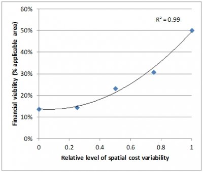
The case study of bench terraces in the Yan River Basin in China shows an important influence of variable investment costs (Figure 1A). When no spatial variability is taken into account, terraces are financially attractive in 13% of the area where they can technically be implemented. This proportion rises to 50% if costs are taken proportionate to the reference slope (Equation 1). Figure 1A clearly demonstrates that the effect of spatial cost variability is not linear; not considering or underestimating the level of variability in costs may hence considerably underestimate potential profitability of bench terracing, whereas overestimating the level of variability of the required investment may rapidly lead to exaggerated viability estimates. Not only does the percentage of the area where the technology can be economically implemented change, but also the locations (results not shown). In absence of slope-related spatial variability, slope does not exert any influence and viability is in this case primarily responding to climatic variation. As the slope dimension is phased in, more and more less sloping land in areas with suboptimal climatic conditions replaces rugged areas with highly suitable climate.
 |
 |
| Figure 1: A. Financial viability of bench terraces in Yanhe river basin under different levels of spatial investment cost variability; |
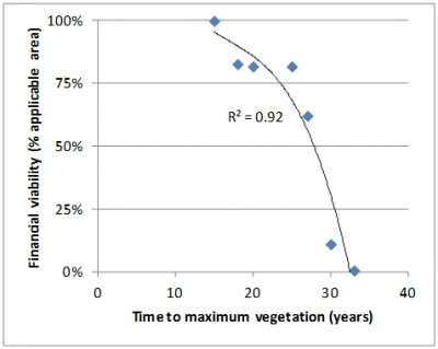
B. Financial viability of gully control with atriplex in Sehoul as a function of time to reach maximum productivity. |
Effect of timing of biophysical effects
The technologies assessed in the DESIRE project included agronomic (e.g. minimum tillage) as well as structural, vegetative and management SLM measures. All measures, but especially the second group, impact on slow soil ecological processes and will gradually improve soil structure and fertility, and hence system productivity. The PESERA model simulates the equilibrium conditions in the with and without technology case. One of the sites where PESERA predicted a particularly large improvement in productivity was in the Sehoul area close to Rabat, Morocco – for gully control by plantation of atriplex (Atriplex halimus). In the standard calculation, it was assumed that production would increase linearly until reaching its maximum value after 20 years - i.e. time to maturity TTM = 20. By employing Equation 2, net present value was calculated for time productivity series with different TTM values (15, 18, 25, 27, 30 and 33 years):
 [2] [2]
Where NPVTTM refers to the net present value of the cashflow series over 20 years for the case with implementation of gully control only; j and t are measured in years and NPV in currency. After calculating NPVTTM values, investment costs and total discounted production in the without case (which remain the same under different TTM values) need to be subtracted. Finally, for evaluation of the effect of TTM, the percentage of cells in the applicability area of the technology is calculated.
Gully control with atriplex in Sehoul, Morocco is not very sensitive to small changes around the assumed 20 years it takes to reach maximum productivity (Figure 11B). However, this is a rough assumption, so we should look further than the short range between 18 and 25 years where the viability of the technology is not affected. When approximating a TTM of 15 years, the viability of atriplex planting rapidly reaches 100% of the applicable area, up from 82% on the stable area from 18-25 year. Even more dramatic is the drop between a TTM of 25 and 30 years, when the technology seizes to viable in more than 60% of the applicable area. The negative slope of the relation flattens of after 30 years, but gully control with atriplex by then remains profitable in only 13% of the area. From this example, it is clear that one would need to be confident of the interval 18-25 years it would take vegetation to reach maximum productivity, outside of which the system becomes very sensitive to the issue of timing.
Discussion of scale issues
In studies of adoption of SLM technologies, plot location is often found to be of importance (e.g. Staal et al, 2002; Noltze et al., 2012). The spatial variation in investment costs of SLM technologies and distance to markets are likely to play a key role, although explicit studies of variations in costs are scarce (e.g. Shively, 1999; Tenge et al., 2005). As Heidkamp (2008), it in a more general context, puts it: “the environment has been largely ignored beyond its treatment as a more or less passive location condition or resource factor input”. Although the illustration of cost differentiation with slope for bench terraces in China provides an example of the susceptibility of outcomes to this factor, the finding that taking variability in investment cost into account leads to a larger viability is specific. In other cases, for example where data is gathered from a relatively cheap experiment in optimal conditions, considering spatial variability factors might lead to reduced levels of predicted viability. Much data on spatial variability of different types of SLM technologies probably exists in design manuals, project documents, and other grey literature. A review of those materials is recommended to define some generic relations that can be used to improve model assessments of SLM.
The timing of biophysical effects has potentially significant influence on viability of technologies. The point version of PESERA allows simulation in time series mode after equilibrium conditions have been established. The grid version of the model, which was used here, lacks this facility. Still, model validation, specifically of timing of effects, is difficult due to interactions and the paucity of long-term field trials which are intensively monitored. Although the illustrative case study had a long term restoration goal, the cumulative effects of annually repeated SLM technologies may also be significant (see e.g. Hobbs et al., 2008). The importance of the temporal dimension in evaluating technologies is clear from the inclusion of a discount factor in CBA. This can work two ways: in the case of technology application, it is important for land users to start reaping benefits as early as possible; but in the without case, ongoing degradation can further affect yield levels (Lal, 1995).
|



 [2]
[2]