A model has been developed for the main bio-physical and socio-economic processes interacting within an agro-ecosystem. This builds on existing experience in combination with results generated within the Study Sites where sustainable land management strategies have been chosen and trialled. Full details of the model are contained in the report which can be downloaded from the link at the bottom of this page.

The inter-linked models described in this report are designed to evaluate the likely biophysical and socio-economic effects of applying remediation strategies selected by stakeholders (in Research Theme 3) at a regional scale, by scaling up results from field trials and secondary data. These models will be applied in all study areas for which there is sufficient data. Additional socio-economic models have been developed for application in a single study site to further explore factors influencing the adoption of remediation strategies by land managers, and the wider effects of adoption on the regional economy.

The report starts by introducing the modelling approaches that are used and explains how these move beyond the state-of-the-art. Next, it shows how the biophysical model proposed for the DESIRE project builds on and extends the Pan European Soil Erosion Risk Assessment (PESERA) model. It also describes a database that is used to assess the effects of soil and water conservation measures on runoff, soil loss and sediment yield at catchment scales.

Desertification policy targets include using sustainable land management strategies to reduce soil erosion and land degradation. In order to determine which strategies for remediation should be implemented where, at least cost, and to make an investment analysis of these strategies for both land users and societies, PESERA outputs are linked to the implementation costs of remediation strategies in each study area. This will result in a cross-site cost-effectiveness analysis and financial cost-benefit analysis, and the latter is also extended with some selected wider economic effects.

This is done using the following steps:

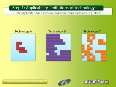
Step 1: First it is necessary to define where each technology can, on biophysical grounds, in principle be applied. Technologies are those selected as promising WOCAT technologies (in Research Theme 3). This is an important step in that it rules out the area where technologies cannot be applied e.g. terraces on steep slopes with shallow soils. Factors considered include: soil depth, slope, land use, climate and distance to streams.
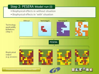
Step 2: The PESERA model is run, taking into account each technology’s potential applicability area, and compared to a case where no technology is applied. This simulates the gradual effects that many technologies may have over time e.g. gradual build-up of soil organic matter, resulting in gradually declining erosion levels and gradually increasing yields. The timing of biophysical effects is crucial for subsequent economic valuation (steps 6 and 11). Thus, this step will produce annual maps for 20 years that show the biophysical effects of each technology.
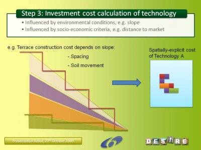
Step 3: WOCAT technology questionnaires currently show only one cost estimate; in reality this will depend on location. We consider two different aspects: environmental conditions (e.g. terrace spacing and hence cost depends on slope) and distance to market. This approach is taken for both investment and maintenance costs.
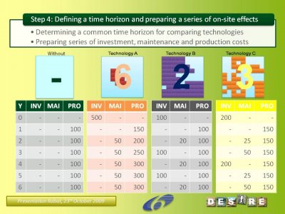
Step 4: The technologies that are being assessed may have different economic lifetimes. Therefore, shorter-lived technologies are assessed over several cycles of re-investment (over the length of time that the longest lived technology is likely to last for). Years of (re-)investment are filled first; maintenance costs are subsequently added for years in between investment. Production costs need also to be considered because application of technologies may lead to a change of land use or use of input (e.g. more labour because of larger harvest).
Step 5: To value effects of a remediation strategy, the following will be assessed on a yearly basis for the lifetime of the technology (or multiple lifetimes): A. Evolution of production output (yield x value) over time B. Evolution of costs of implementing the technology and land use associated with it C. Evolution of production output (yield x value) as it would develop were the mitigation strategy not applied D. Evolution of the costs associated with the land use in this ‘without’ case For each year, the net result can then be calculated as [A-B-C+D] (note that benefits and costs may vary both in space and time).
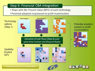
Step 6: The annual cash-flows of Step 5 are subsequently used in a Financial Cost-Benefit Analysis (FCBA). An important issue in FCBA is discounting, i.e. introducing an interest rate that depreciates costs or benefits occurring in the future relative to those felt now. Summing discounted cash-flows gives the Net Present Value (NPV) for each technology. For each grid cell, one of the following three possible outcomes will apply. The technology with highest NPV will be selected (when positive) (the adoption grid shows a possible configuration of technology A, B and C). No technology will be selected if all NPVs are negative (i.e. white pixels in potential adoption grid). No technology will be selected if no technology is applicable in the area (blue cells in adoption grid.
Step 7: In this step, the socio-economic analyses done so far will be contrasted against the biophysical effects of technologies according to PESERA. When the investment costs of a technology are compared to its effectiveness to reduce land degradation problems, a policy-relevant indicator results, as land users may need assistance to cover the investment costs. A further refinement is made when substituting the total non-discounted cashflow of a technology for the investment costs: in this case private returns are subtracted, and the resulting indicator shows whether, in principle, public resources are needed to complement private returns in order to cover the costs for land users of implementing technologies. Finally, by using NPVs in this analysis, it becomes clear whether the timing of benefits relative to the incurrence of costs is appreciated by the land user; if this is not the case, subsidies may be required to persuade the land user to implement the technology. In all cases, policy-makers should keep track of the effectiveness of measures. Two types of evaluating the effectiveness are possible: a) defining a maximum level of acceptable land degradation that should be met in all grid cells, and b) defining an aggregate level reduction target to determine where the most effective interventions can be made at minimum cost.
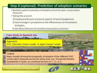
Step 8: Adoption of mitigation measures as defined in Step 6 is solely based on profit maximization. Land users may in reality have more varied reasons to adopt or not to adopt soil and water conservation measures. For the Spanish case study site, we will do a detailed study of spatially explicit adoption, or in other words, determine where land users have implemented what measures. In this case study, a questionnaire will yield the necessary data for developing a discrete choice model and agent-based model integrated with GIS. This step will yield more reliable adoption maps for scenario studies that can be used instead of the approach of Step 6.
Step 9: This PESERA model run differs from the first run in that it will be based on a configured technology adoption map (i.e. produced in Steps 6 or 8) instead of separate runs for each technology taking into account its applicability limitations (Step 1). It will be interesting to map PESERA output data for their own sake, either by visualizing the final physical impact of land mitigation strategies or as a reduction relative to the without situation. Such output maps can be used to inform policy development scenarios (Step 12) and to integrate these effects in a CBA including selected wider economic effects (Step 11). Apart from maps, also aggregate accounts for each of the output variables can be elaborated, for example showing the regional average reduction of soil erosion as a result of the predicted adoption of SLM technologies.
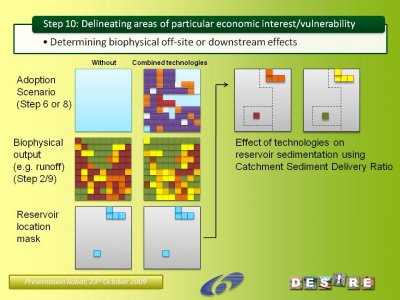
Step 10: PESERA treats grid cells as independent units, so it cannot be used directly to assess off-site effects. This step details how PESERA can still be used to assess off-site effects in an indirect fashion. For each effect the area of interest will be delineated and its magnitude assessed based on transfer functions (currently only reservoir sedimentation).
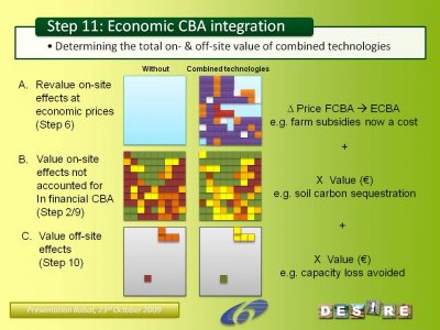
Step 11: The financial CBA (FCBA) of Step 6 provided a valuation from an individual farmer’s perspective. In this step, an economic CBA (ECBA) is made, valuing the combined effects of regional adoption patterns (Step 6/8) from a societal perspective, taking into account issues such as off-site effects and the cost of providing subsidies. For example, an ECBA would include the effect of SLM technologies on reducing reservoir sedimentation, an effect that is not considered by individual land users. As reservoir construction requires considerable (public) investment, preventing the loss of reservoir capacity and in this way prolonging its lifetime, it is an important off-site benefit for society.
Step 12: Once Steps 1-11 have been set-up, the model can be used for policy evaluation or policy design. Such policies can: Affect farmer’s valuation of effects, e.g. by increasing agro-environmental subsidies for adopting certain measures (these effects will feedback in Steps 6/7 and require reassessing subsequent steps as well) Enforce adoption of technologies (Step 8) Stimulate/enforce environmental targets (Step 3/4)

Finally, the report describes models that have been developed for application in Spain to investigate the regional economic effects of adopting different remediation strategies (using regional economic modelling), and determine what factors influence land managers to adopt different remediation strategies and change land use under different future scenarios (using Agent-Based Modelling).

This modelling approach contains a number of important novelties. For example:

• The approach overcomes a number of challenges to incorporate inputs from multiple stakeholders in very different contexts into the modelling process, in order to enhance both the realism and relevance of outputs for policy and practice.
• A number of modelling approaches are being applied to the mitigation of land degradation for the first time to provide novel insights. For example, site-selection modelling is being applied to land degradation mitigation to enable landscape-scale assessments of the most economically optimal way to attain of environmental targets.
• There have been few attempts to use Cost-Benefit Analysis to investigate the spatial variability of the profitability of SWC measures, which may have important implications for the adoption of measures across landscapes and their consequent environmental effects.
• For the first time, regional (input-output) economic models are also being used to consider the effects of land degradation mitigation on the regional economy.
• By linking (Agent-Based) models of human behaviour to models that describe the wider regional economic and biophysical implications of people’s actions, it may be possible to better understand how people are likely to respond to environmental change, and how their responses in turn are likely to influence their environment. Such models may offer us the opportunity to explore how land managers might react to different future policy options and provide ways to make refinements to policy design that can more effectively achieve environmental sustainability goals.

The fact that much of this is being done for multiple study areas based on data gathered by a collective effort between researchers and local stakeholders makes the approach truly unique. Cross-site scaling-up of the model will for the first time be able to provide estimates of the global impact of land degradation mitigation, built on local realities.

More details ... read on-line or download the full report
	WP5.1 PESERA-DESMICE Land management evaluation model
	WP5.1 PESERA-DESMICE: Land management evaluation model [2.26 MB]