|
The PESERA-DESIMCE model output for each study site is presented in a generic format which is explained here, together with any assumptions made in preparing the results.
Study site details
 |
The front page for each study site starts with a short facts section and overview map of the study site. The facts include a one-sentence description of the study site, the coordinates (latitude, longitude) of either the boundaries or center point of the study site and size of the area. Together with the overview map, these facts help the reader to locate the area. Note that none of the subsequent maps of model results offer location or coordinates – hence the importance of this front page section. |
Further details include data on altitude, precipitation levels, temperature range, land use, population and perceived most important degradation processes and drivers. This information is mostly summarized from »Compilation & synthesis of study site descriptions. Note that for model analyses, DEMs and spatial data sets of climate, soil and land use were used – the details provided here are just to give a snapshot view of study site characteristics. The number of inhabitants here reported is used in calculations such as per capita food production.
Overview of scenarios
 |
The front page also lists the scenarios run for the particular study site. Their number varies, e.g. depending on the number of technologies tested or for which there was sufficient data, or the existence of policy options. |
Where scenarios relate to technologies included in the DESIRE WOCAT database the corresponding reference number is given (e.g. CPV01).
Baseline scenario
 |
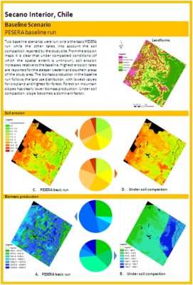
The PESERA baseline run shows model results for the study site under current conditions (see »PESERA-DESMICE model for technical details). Usually, only one set of output maps is shown here. However, sometimes, such as in this Chilean case, there is a lack of clarity over current study site conditions – in this case the level of compaction. Hence two baseline output maps are shown, one for uncompacted and one for compacted conditions.
The first map (top right) shows a landforms map for the study area which is produced by a DESMICE submodule from the study site DEM. Not only is the landforms map frequently used to determine applicability limitations (as per WOCAT records), it is shown here as it gives a good overview of the topographic conditions of the study site.
|
Soil erosion maps are presented with fixed classification of soil loss, so that one can compare the severity of land degradation across study sites. To note that PESERA soil loss estimates are field-based, i.e. there is no routing of sediments through stream networks. In the Portuguese study sites, instead of soil erosion, maps of fire severity index (FSI) are depicted, as the local degradation problem is susceptibility to and occurrence of wildfires.
Biomass production maps do not have a fixed legend, as variations between study sites are too large for a single classification to be relevant. Within a study site, the map can show nuances in productivity caused by environmental gradients as well as the sometimes large variation between different land uses – e.g. arable land versus forests. The units of biomass production are kg/ha or ton/ha and include whole-plant biomass, not just yields. A harvest index is required to calculate the latter.
| Box 1: Use of pie charts and use of background colour for no data
The model results are frequently presented in a dual format: as a distributed feature on a map and as a pie chart. Both formats are interrelated. The pie charts can be helpful to quickly assess the distribution of the characteristic depicted over a classification – which is sometimes difficult to see on the map. Pie charts are in principle drawn for the area for which data is shown on the map; i.e. the black background in the maps above represents areas with no data, which are consequently ignored in the pie charts. One exception are the green/black applicability limitation maps where green stands for ‘the technology is applicable’ and black for ‘not applicable’ (see an example in the next section about Technology scenarios). Background colours for no data sometimes vary per map for reasons of visibility – they can be recognized by bearing no association to the legend colour scheme.
|
Technology scenario
 |
A technology scenario presents the model output for a specific remediation option. They form the core of the scenario simulations, as policy, adoption and global scenarios are based on them. The description starts with a number of facts or assumptions that were used in the simulations. These may pertain to the situation under the current conditions ('without' case), the situation after implementation of the technology, or both. Costs and prices are given in local currency and Euros to facilitate cross-comparison between sites. All numbers are either based on reports by study sites (WOCAT database), secondary sources or in some cases derived from other study sites with comparable conditions. Applicability limitations show the share of the study area where the technology can, in biophysical terms, be implemented. |
Soil erosion maps compare annual soil erosion in the with and without situation. For the Portuguese study areas, where wildfires are the main degradation problem, erosion maps are replaced with fire severity index (FSI) maps. The impact of the technology on biomass is here considered especially as a degradation mitigation outcome and hence focuses on total biomass rather than yields (one can multiply values with a harvest index if given to arrive at yield levels; or refer to the global food production scenario). Shown are a map of the percentage of biomass increase relative to current conditions and total biomass after implementation of the technology.
Economic viability maps come in two flavours:
- For agronomic measures that need to be repeated annually as part of the production cycle, the maps present the outcome of a partial budget analysis of the difference of costs and benefits in the with and without situation.
- For technologies requiring investment (also if only in kind) and where benefits accrue only after a certain period, cost-benefit analysis (CBA) is applied and includes the use of a discount factor. The map in this case presents the Net Present Value (NPV) of the investment.
|
Box 2: Assumptions for economic viability calculations
Financial analysis of the technology under consideration is an essential element of each technology scenario, and is revisited in any policy scenario (if applicable). Exact cost and benefits are hard to define. Care has been taken to err on the conservative side so that the assessment does not paint a rosy picture of the technology. Here are some of the most important assumptions made and residual issues that need to be taken in mind when using the presented figures:
- A profitability or NPV of 0 is deemed to be the minimum required for financial viability of a technology. It is acknowledged that many factors come into play for a land user to decide to implement a technology, but if a technology does not at least maintain the current financial status quo the technology is not attractive.
- In the technology scenario, all costs are assumed to be incurred by the land user (or other decision-making entity). Any subsidies or other forms of incentives are excluded from the analysis. In the WOCAT terminology, the results thus reflect the financial attractiveness of a technology for spontaneous adoption.
- It appeared to be difficult for study sites to estimate spatial variation in investment costs of technologies. Environmental variations (e.g. with slope steepness) are taken into account for structural measures such as terraces, but distance to source areas and markets was not taken into account in the analyses.
- While the temporal dimension of changes in productivity is crucial for land users, PESERA assessments of technologies produce equilibrium outputs. The time lag to arrive at these equilibrium conditions is not explicit. In the case of some management measures, especially those implemented on severely degraded lands, it may take a very long time to arrive at equilibrium conditions. Linear trends are assumed in these cases, with equilibrium conditions assumed to be reached after 20 years.
- Similarly, current conditions are assumed to be at equilibrium. No ongoing productivity decline due to progressing degradation is considered in the without case.
- Where perennial crops are planted as part of a technology, progression of productivity is set according to local and species-specific trends.
- Some structural technologies harvest water or accumulate land from a larger area. In these cases, a conversion factor such as a catchment to cropped area ratio (CCR) has been assumed. Conditions in the catchment area are assumed to remain constant after implementing the technology.
- In the specific case of Portuguese study sites, where technologies are intended to mitigate risk of wildfire occurences, analyses have been performed based on actual fire outbreaks between 2000-2009 for which spatial data were available. In these cases, a single financial viability estimate is given as the application of the technologies is not assessed from an individual land user perspective but for a municipality as a whole.
- All financial analyses are of course sensitive to price fluctuations. Although no sensitivity analyses are performed, one of the most difficult assumptions is the price of labour (opportunity) costs. All analyses have duly priced all labour input at the going daily wage rate in the study areas. Land users are known to accept lower return to labour in several circumstances (slack season, conservation works around the home in spare time, etc.) so that fnancial viability maps can be regarded as conservative estimates.
|
Policy scenario
 |
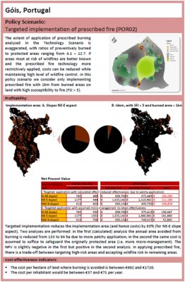
Policy scenarios are presented for any incentive or strategy that could help to improve the viability and/or extend the adoption of a technology with the final goal of enhanced mitigation of land degradation. Most frequently, policy scenarios assess the cost-effectiveness of subsidies to reduce investment costs to implement a technology for land users (e.g. an incentive in the form of a 50% reduction is often presented). The policy scenario starts with a description of the issue and the type of incentive/strategy to be evaluated. Subsequently, the profitability of the technology with and without the policy is compared. In the Góis example used here, estimates for profitability are given for the entire area and are not spatially-explicit. Hence, the comparison is made in a table format and instead, the changes in the area subjected to prescribed fire are depicted in maps. |
Finally, cost-effectiveness indicators are presented to assess the cost of the policy measure (from a public, or governance perspective) in relation to the environmental benefit obtained. Cost-effectiveness can be expressed in monetary units per ton of soil loss prevented, or per hectare of land saved from burning.
Adoption scenario
 |
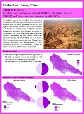
Adoption scenarios are presented where multiple technologies with partially overlapping applicability areas are being assessed. The purpose of the adoption scenario is to provide a summary overall view of the spatial arrangement of the possible mitigation options, and the adoption patterns if it is assumed that in each cell, the most profitable technology (i.e. the one with the highest NPV) is selected. This assessment is made for all technology scenarios (‘without policies’) and all policy scenarios combined (‘with policies’). For many study sites, only a single technology scenario was run, or different technologies had mutually exclusive applicability areas. In such cases, there would be no added value in presenting an adoption scenario, which is hence not elaborated. |
Global scenario
The final type of scenario takes a reverse approach to the policy scenario. Instead of asking the question what the effectiveness of a policy is, it considers the technical capabilities of the remediation option(s) in creating impact across the study area, and then provides an investment requirement. The objective of this analysis is not so much a local analysis, but to provide a global comparison of potential impact – hence the name ‘global scenario’.
 |
Two types of global scenarios are presented:
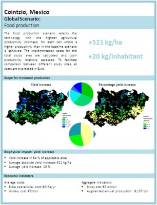
- Scope for increased food production, assessing how much more food could be produced in an area if desertification remediation strategies were adopted to the maximum extent (insofar as they enhance crop production); and
- Scope for minimizing land degradation, assessing by how much soil erosion could be curbed if effective remediation strategies were fully implemented.
|
In both cases, the absolute and percentage improvements relative to current conditions are presented. Note that for food production, yield increases are reported rather than biomass increases. For erosion reduction, negative rather than positive numbers are effective and colour coding for soil erosion reduction classes have been inverted to illustrate this fact.
Biophysical impact and economic indicators are subsequently provided. These are also used to calculate the main indicators presented in the top-right corner: yield increase per hectare and per capita for food production scenarios, and erosion reduction per hectare and cost per ton of soil prevented from eroding for land degradation minimization scenarios.
|
Box 3: Food production increases
Increased cereal yields, even of different crops, are deemed to be directly comparable across study sites as they have similar calorific content. Yield increases of other crops, such as olives and apples, are also provided but not included in cross-site analysis due to their non-staple character. Still other production increases, such as rangeland productivity having an impact on livestock production, and agave production for alcohol distilling, have not been reported here. |
Concluding remarks
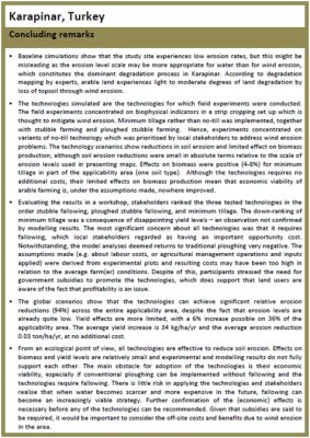
The final page of each study site report recaptures the main points of the analyses, and provides a narrative for the specific study site context and processes. Where possible, reference is made to other DESIRE results such as:
 |
- The expert mapping of land degradation in »Mapping desertification extent is compared to the PESERA baseline run;
- Technology scenarios are assessed against experimental results »Local field experiment results and conclusions;
- Stakeholder opinion about technologies and its evolution in time between »Selecting strategies for field testing and evaluation of experimental results by stakeholders is discussed in relation to model results;
- Local policies (»Drivers and policy context) and stakeholder opinion about how to promote sustainable land management are revisited when discussing results of policy scenarios
- Adoption and global scenario results are presented with a view of supporting recommendations for extension and policy.
- Finally, an overall conclusion is given which refers to the general context of environmental change and the feasibility of the remediation options considered to build resilience, as well as any remaining research before such recommendations can be made.
|
|

