PESERA-DESMICE: Land management evaluation model

Table of Contents

1. Authors
2. Summary
3. Acronyms
4. Introduction
5. Coarse-scale model description
   1. The PESERA model: summary
   2. Alternative approaches to assessing soil erosion
   3. Process representation in PESERA
   4. Extensions of PESERA
   5. Adapting PESERA
   6. Assessment at catchment scales
6. Cost-effectiveness modelling
   1. Step 1
   2. Step 2
   3. Step 3
   4. Step 4
   5. Step 5
   6. Step 6
   7. Step 7
   8. Step 8
   9. Step 9
   10. Step 10
   11. Step 11
   12. Step 12
7. Agent-Based modelling in Spain
   1. Phase 1
   2. Phase 2
   3. Phase 3
   4. Phase 4
   5. Phase 5
   6. Phase 6
8. Input-Output modelling in Spain
   1. Model construction
   2. Scenario analyses
9. References

Step 2

Step 2: PESERA Model run 1

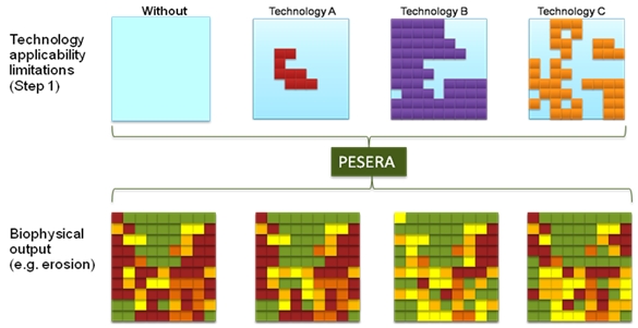
The physical effects of implementing the technology can now be evaluated using the PESERA model. This should be done separately for each technology, taking into account its potential applicability area (step 1). The resulting output should be compared to the situation without implementing any (additional) technology. This output, which can be considered the technically feasible mitigation of land degradation, provides a meaningful PESERA output, but is not yet based on socio-economic variables. From PESERA runs, which include stochastic climate events, temporal trend series will be constructed that will simulate the gradual effects that many technologies may have (e.g. gradual build-up of soil organic matter, resulting in gradually declining erosion levels and gradually increasing yield levels). Timing of biophysical effects is crucial for subsequent economic valuation (steps 6 and 11). Thus, this step will produce annual output maps for a time series of 20 years (assuming no technology will have an economic lifetime longer than that, see step 4).

The PESERA model, adapted to evaluate the biophysical effects of land degradation remediation technologies (section 2) is a grid-based model that can be applied at a grid cell size of 0.01 - 1 km². Table 3.1 shows a list of typical output variables generated by PESERA. The cost-effectiveness model will produce output at the same resolution as PESERA. However, some intermediate results may be available at finer (or coarser) resolution. Where this is the case subgrids (or supergrids) will be defined that can be generalized in the final resolution.

Table 3.1: Typical output variables for each cell in the PESERA model (Kirkby et al., 2008)

Data sources: 1) PESERA input data; 2) raster layer showing potential applicability of each technology (step 1)

Intermediate products: annual maps of PESERA output values for with and without situations for each relevant technology in each site (Figure 3.3)

Figure 3.3: Example output maps for the first PESERA run for different with and without situations