PESERA-DESMICE: Land management evaluation model

Table of Contents

1. Authors
2. Summary
3. Acronyms
4. Introduction
5. Coarse-scale model description
   1. The PESERA model: summary
   2. Alternative approaches to assessing soil erosion
   3. Process representation in PESERA
   4. Extensions of PESERA
   5. Adapting PESERA
   6. Assessment at catchment scales
6. Cost-effectiveness modelling
   1. Step 1
   2. Step 2
   3. Step 3
   4. Step 4
   5. Step 5
   6. Step 6
   7. Step 7
   8. Step 8
   9. Step 9
   10. Step 10
   11. Step 11
   12. Step 12
7. Agent-Based modelling in Spain
   1. Phase 1
   2. Phase 2
   3. Phase 3
   4. Phase 4
   5. Phase 5
   6. Phase 6
8. Input-Output modelling in Spain
   1. Model construction
   2. Scenario analyses
9. References

Step 9

Step 9: PESERA Model run 2

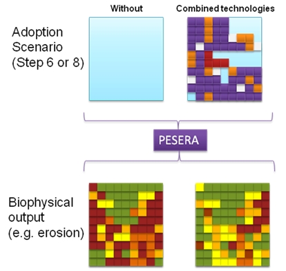
When a technology adoption map (step 6 or 8) is ready, this can be fed back into PESERA to evaluate the impact on output variables. In this second PESERA model run, grid cells will either feature the technology with the highest NPV (if the technology adoption map from step 6 is used) or the technology as predicted according to the adoption pattern simulated in step 8. This PESERA model run thus differs from the first run in that it will be based on a configured technology adoption map instead of separate runs for each technology taking into account its applicability limitations. It will be interesting to map PESERA output data for their own sake, either by visualizing the final physical impact of land mitigation strategies or as a reduction relative to the without situation. Such output maps can be used to inform policy development scenarios (step 12) and to integrate these effects in a CBA including selected wider economic effects (step 11). Apart from maps, also aggregate accounts for each of the output variables can be elaborated.

Data sources: 1) PESERA input data; 2) map with spatially explicit adoption of technologies (step 6/8)

Intermediate products: annual maps of PESERA output values (Figure 3.8)

Figure 3.8: Example output maps for the second PESERA run for combined technologies and without situation