PESERA-DESMICE: Land management evaluation model

Table of Contents

1. Authors
2. Summary
3. Acronyms
4. Introduction
5. Coarse-scale model description
   1. The PESERA model: summary
   2. Alternative approaches to assessing soil erosion
   3. Process representation in PESERA
   4. Extensions of PESERA
   5. Adapting PESERA
   6. Assessment at catchment scales
6. Cost-effectiveness modelling
   1. Step 1
   2. Step 2
   3. Step 3
   4. Step 4
   5. Step 5
   6. Step 6
   7. Step 7
   8. Step 8
   9. Step 9
   10. Step 10
   11. Step 11
   12. Step 12
7. Agent-Based modelling in Spain
   1. Phase 1
   2. Phase 2
   3. Phase 3
   4. Phase 4
   5. Phase 5
   6. Phase 6
8. Input-Output modelling in Spain
   1. Model construction
   2. Scenario analyses
9. References

Step 6

Step 6: Financial CBA integration

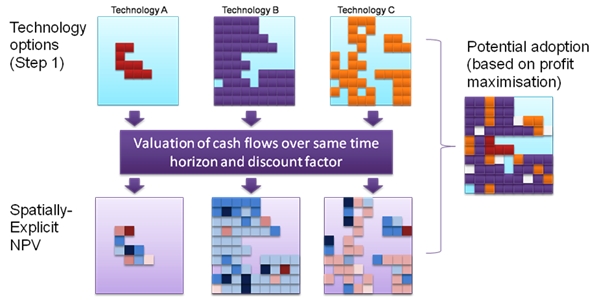
The steps 1-5 allow quantification and valuation of all effects considered, for each technology separately. In this subsequent step, a formal decision based on farmer profit maximisation will be made for each grid cell. This entails applying a discount rate to the annual cashflows generated by each technology, and determining Net Present Values (NPV) and Internal Rates of Return (IRR). NPV is obtained by summing discounted cashflows. The IRR is the discount factor at which the investment becomes attractive (i.e. at which the NPV is 0). The discount factor can be established from the cost farmers incur to borrow money. The rationale behind this is that borrowing money to invest should at least yield the sum borrowed plus interest and transaction costs. Adoption of the most profitable technology (based on NPV and/or IRR) will be assumed (this may also include non-adoption, if none of the technologies evaluated result in sufficient tangible benefits for the farmer). For each grid cell, one of the following three possible outcomes will therefore apply:

1. The technology with highest NPV will be selected (when positive);
2. No technology will be selected if all NPV's are negative; and
3. No technology will be selected if no technology is applicable in the area.

The above standard method evaluates the profitability of investment alternatives when capital and land are the scarcest factors. This may not always be the case. The following additional analyses can therefore be undertaken:

1. For many farmers labour may be a critical factor, and return to labour rather than return to capital investment is important. Especially where off-farm work opportunities exist, return to labour should be considered in relation to the opportunity cost of labour. If this comparison turns out negative, then investing in the land is doubtful, and abandonment would be a sensible strategy
2. Labour itself may also be limiting. In areas with ample land availability and characterised by the absence of a labour market (especially when land is held as a common property resource), it could be assumed that technologies would be adopted in the areas of highest profitability until available labour resources are exhausted. The model can handle this by attributing finite labour pools to source areas (villages) which will impose a limit on the adoption of technologies

These additional analyses can be performed optionally after the general analysis has been completed.

Data sources: 1) annual cashflow series (step 5); 2) discount factor; 3) (optional) additional data for labour opportunity costs or labour availability.

Intermediate products: 1) raster map with spatially explicit IRR/NPV of each technology (Figure 3.6); 2) raster map with combined constructed adoption of all technologies (Figure 3.6); 3) raster map with spatially explicit IRR/NPV of adopted technologies.

Figure 3.6: Construction of maps with spatially-explicit NPV of each technology (bottom) and resulting adoption map (right)